I recently had the opportunity to present my research in a poster session at the AGU conference in San Francisco. My most recent work was the development of interpolated surfaces of temperature and humidity for BORR using observations from our wireless sensor network. Up to that point, I had been relying on the automap package for R to systematically fit semivariograms to monthly-averaged temperature and humidity data. My rationale was that since the range of temperature or humidity and the strength of the elevation trend varied significantly from month to month, any patterns of spatial correlation could also change. Additionally, I wanted to code my procedure to work with arbitrary data. An autofitting algorithm was therefore necessary to construct the semivariograms, and the autofitVariogram function seemed to suit my needs.

Developing the semivariogram is perhaps the most important step in the kriging process, but I adopted a rather cavalier attitude about it in my eagerness to make pretty pictures. Initially, I spent little time familiarizing myself with the optional arguments and assumed the defaults would be good enough. This resulted in a couple of funny-looking maps and some raised eyebrows at my poster session. The problem was that in some cases, autofitVariogram produced semivariograms with very steep ranges and flat sills, such as the one below for average maximum humidity in April:

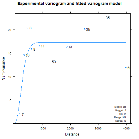
It is pretty obvious that the autofitted theoretical semivariogram is not really capturing the true nature of the experimental semivariogram. For one thing, it looks like the higher distance intervals may be throwing off the fitting algorithm. For another, the uneven binning may be causing problems when the kriging weights are computed. The first step is to check the documentation for autofitVariogram (also available here) to see how it defines the bins. By default, autofitVariogram requires that each bin contain at least five points, and the function provides the merge.small.bins and min.np.bin named arguments (via miscFitOptions) to allow user customization of the bins. But hang on, here’s how it works:

the function checks if there are bins with less than 5 points. If so, the first two bins are merged and the check is repeated. This is done until all bins have more than min.np.bin points.

This presents a problem: if there are small bins in the middle of the data, all the bins to the left will get merged first. This could be an issue when observations are sparse or clustered in certain regions. A better method might be to resize the bins (e.g. by maintaining bins of equal width) so that each contains the minimum number of points. Alternatively, one could define the bins so that each contains the same number of observations. The next step is to check out the source code to see how autofitVariogram defines the bins by default. In particular, we are interested in the definition of the variable boundaries, which is passed as a named argument to the function variogram (from the gstat package) during the fitting process.

# Create boundaries
longlat = !is.projected(input_data)
if(is.na(longlat)) longlat = FALSE
# 0.35 times the length of the central axis through the area
diagonal = spDists(t(bbox(input_data)), longlat = longlat)[1,2]
# Boundaries for the bins in km
boundaries = c(2,4,6,9,12,15,25,35,50,65,80,100) * 
             diagonal * 0.35/100

As shown above, autofitVariogram defines boundaries (the distance intervals which define the bins) as 2%, 4%, 6%, …, 100% of about 1/3 the diagonal of the box spanning the sample locations (defined using the spDists function from the sp package). The rationale behind defining the bins in this way is not apparent from the automap documentation, but limiting the highest interval to 35% of the diagonal is consistent with the default behavior of variogram.

There are two important arguments to variogram that we are ignoring here: width and cutoff. The argument width seems to match our equal-width binning idea. We can provide our own value of cutoff to exclude the larger distances. Unfortunately, the gstat documentation doesn’t specify what happens when we provide cutoff and/or width in addition to boundaries.

No matter what, trying out different binning methods requires modifying autofitVariogram’s definition of boundaries. For using equal-width bins while maintaining a minimum number of points, We can skip the definition of boundaries entirely. We instead iteratively increase the value of width (thereby decreasing the number of bins) until every bin contains at least the number of points defined by min.np.bin. Of course, this only works if either an initial bin width (via a new named argument, init.width) or a starting number of bins (through another named argument, num.bins) is supplied.

if(miscFitOptions[["equal.width.bins"]]){
  if(verbose) cat("Using equal-width bins...\n\n")
  if('width' %in% names(list(...))) error('Cannot pass width when equal.width.bins = TRUE. Supply "init.width" to miscFitOptions istead')
  # redefine diagonal if cutoff was supplied
  if('cutoff' %in% names(list(...))) diagonal <- list(...)[['cutoff']]
  # user must supply either width or num.bins
  if(!'init.width' %in% names(miscFitOptions)){
    width <- diagonal/miscFitOptions[['num.bins']]        
  } else {
    width <- miscFitOptions[['init.width']]
  }
  if(verbose) cat("Checking if any bins have less than ", miscFitOptions[["min.np.bin"]], " points, merging bins when necessary...\n\n")
  while(TRUE){
    if(!is(GLS.model, "variogramModel")) {
      experimental_variogram = variogram(formula, input_data, width = width, ...)
    } else {
      experimental_variogram = variogram(g, width = width, ...)
    }
    if(length(experimental_variogram$np[experimental_variogram$np < miscFitOptions[["min.np.bin"]]]) == 0) break            
    # increase width by 10% and try again
    width <- width*1.1
  }
}

To implement this code, the user simply passes equal.width.bins = TRUE in miscFitOptions. Note that variogram does some of its own binning, so we won’t end up with bins of exactly equal width. By removing autofitVariogram’s definition of boundaries we avoid ambiguous behavior by never passing both boundaries and width in a call to variogram. We can easily preserve the old behavior by adding another named argument, e.g. orig.behavior. This also gives the user the ability to pass their own definition of boundaries to autofitVariogram.

How about using equal-count bins? We can do this pretty easily by redefining boundaries. We implement this method with the named argument equal.np.bins.

if(miscFitOptions[["equal.np.bins"]]){
  if(verbose) cat("Using bins of equal observation counts...\n\n")
  if('boundaries' %in% names(list(...))) error('Cannot pass boundaries when equal.np.bins is TRUE.')
  if('cutoff' %in% names(list(...))) diagonal <- list(...)[['cutoff']]
  # get a sorted list of distances 
  dists <- sort(spDists(input_data))
  # apply the cutoff and remove zeros
  dists <- dists[dists < diagonal &amp; dists &gt; 0]
  # split the data into bins based on number of observations
  if(is.na(miscFitOptions[['num.bins']])){
    # compute number of bins based on the minimum number of observations per bin
    miscFitOptions[['num.bins']] <- floor(0.5*length(dists)/miscFitOptions[['min.np.bin']])
    cat("num.bins not supplied. Setting num.bins = ", miscFitOptions[['num.bins']], '\n\n')
  }
  cat("checking bins, decreasing num.bins if necessary... \n")
  while(TRUE){
    # compute interval based on the number of bins
    interval <- length(dists)/miscFitOptions[['num.bins']]
    # define boundaries
    boundaries <- rep(NA, miscFitOptions[['num.bins']])
    for(i in 1:miscFitOptions[['num.bins']]){
      boundaries[i] <- dists[round(i*interval)]
    }
    if(length(boundaries == length(unique(boundaries)))) break
    # reduce number of bins
    miscFitOptions[['num.bins']] <- miscFitOptions[['num.bins']] - 1 
  }
  if(!is(GLS.model, "variogramModel")) {
    experimental_variogram = variogram(formula, input_data, boundaries = boundaries, ...)
  } else {
    if(verbose) cat("Calculating GLS sample variogram\n")
    g = gstat(NULL, "bla", formula, input_data, model = GLS.model, set = list(gls=1))
    experimental_variogram = variogram(g, boundaries = boundaries, ...)
  }
}

Of course, this won’t create bins with exactly the number of points specified unless the user happens to supply a multiple of the number of distance pairs.

Let’s try out the binning methods now. The first variogram uses equal-width bins, initially of width 500. The second variogram specifies 13 bins containing approximately equal numbers of observations.

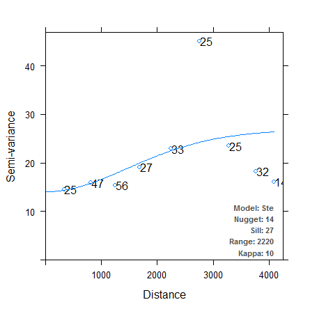
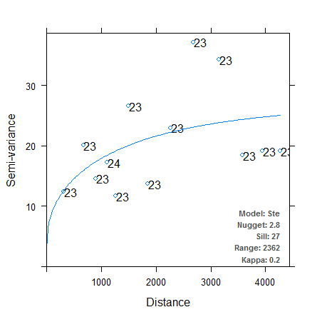
It is immediately clear that in both cases, the autofitted theoretical variogram better approximates the experimental data. We have managed to make the autofitting algorithm more robust just by changing the binning process, although which method provides the “better” fit is still up for debate. There are other arguments we can pass to variogram (e.g. cutoff, cressie, and PR) to further finesse our theoretical semivariograms, and we could also try fitting power models or nested models. I’ll leave those techniques for a future post. For now I’ve included a direct link to the source code for my modified version of the autofitVariogram function here. Incorporate the function into your R code using source, or reassign it to the autofitVariogram function in the automap package. This function hasn’t been tested outside my own purposes, so check the source code and use at your own risk!