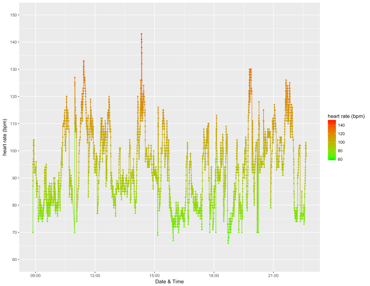
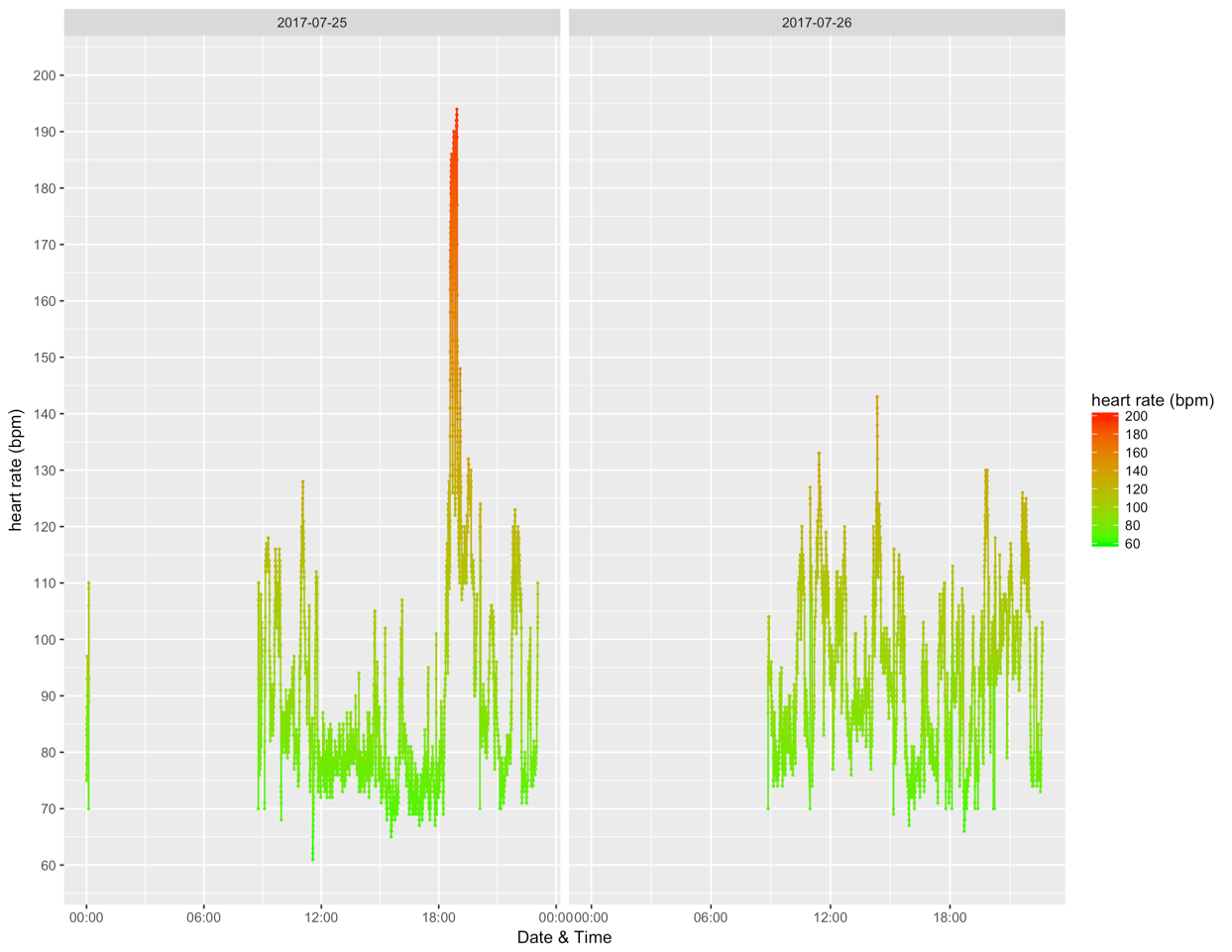
Getting your detailed Fitbit heart rate data with R: a guest post

In this guest post, Tiffany shows us how to access the fitbit API to explore and visualize our personal biometric data.

I have POTS; to keep better track of my actual heart rate, I got a Fitbit Alta HR. I’ve read many terrible reviews for wrist heart rate monitoring with Fitbits, but I have tiny wrists and the Alta HR was the smallest I could find with a nice form-factor. I ordered it on Amazon fully expecting to return it, and I almost did when I realized that the heart rate data is displayed to you in the app and on the website dashboard as a FIVE MINUTE AVERAGE, when it takes and records data way more often (1+ times per minute). Why fitbit decided this was the best thing to do, without giving you the option to change it, is beyond me – especially considering the wrist tracker itself shows you the rapid measurements real-time. I dug around a bit and found that Fitbit has an open API, and working off some old code I found, along with examples for the new Fitbit personal data authorization, I worked out a method to access the detailed heart rate dataset.

The difference between the five-minute averaged dataset and the actual dataset is ridiculous. Peak heart rate during a run, displayed on my tracker, was in the 190’s. Peak heart rate returned by the Fitbit app? 170. Ridiculous. And useless for those of us who have POTS and are susceptible to rapid changes in heart rate. When I pulled the detailed Fitbit datset, it accurately returned every measurement that I noticed while running (plus more). The only issue I noticed is that the Alta HR occasionally doesn’t capture that peak jump right after standing that can occur for less than 30 seconds. (at least in my case), but does regularly pick up the higher heart rate within the minute. Overall, it does a pretty good job and I am pleasantly surprised. I’ve checked my pulse manually (and with a bp cuff) during exercise and throughout the day and it was only 1-2 bpm off from the Fitbit.

The heart rate data can only be downloaded in one-day chunks (i.e. 12AM - 11:59PM on any given day). Here’s the method for how to get the data yourself using R:

1. Create an empty google sheet and name it whatever you want.

Leave this open as a tab.

2. Register an app.

Head to the fitbit developer website and sign in. Then click “Register an App” at the top:

enter whatever you want for Application name and description
in the application website box, paste the URL of your google sheet from Step 1
for organization put “self”
for organization website put the URL of your google sheet from Step 1
for OAuth 2.0 Application Type select “Personal”
for Callback URL put in http://localhost:1410/
for Default Access Type select “Read Only”
click “save”

You should now be at a page that shows your

OAuth 2.0 Client ID
Client Secret

Save these two numbers!

3. Open an R session

In R, define your user tokens, the location on your machine to store the data and the day you want to download data for. The code below assumes you want yesterday’s data. If you don’t, remove the -1 from the date-to_download line and it will download what is available for today. If you want some day in the past, enter the date in the format "YYYY-MM-DD" (include the quotes).

##PARAMETERS###

#remove -1 for today, or enter date as "YYYY-MM-DD" (with quotes) for any other day
	
date_to_download <- as.character(Sys.Date()-1) 
	
##enter your personal key and secret here, leave them in quotes!
##example -- change to:  client_id <- "123ABC"
	
client_id <- "client_id"
secret <- "secret"
	
###path to save CSV and plot
### example -- change to: outpath <- "C:/Users/JaneDoe/Desktop/HeartRate"
	
outpath <- "path"
	
#################

Next, load some packages that we will use to process and visualize the data. Uncomment (delete the #) the top four lines if you haven’t installed these packages yet:

#install.packages("ggplot2")
#install.packages("jsonlite")
#install.packages("httr")
#install.packages("plyr")
library(jsonlite)
library(httr)
library(ggplot2)
library(plyr)

Finally, download the data and visualize it. Don’t change anything here unless you want to tweak the code:

##make no changes below here, unless you know what you're doing.
dir.create(file.path(outpath, "plot"))
dir.create(file.path(outpath, "data"))
fbr <- oauth_app('FitteR',client_id,secret)
accessTokenURL <-  'https://api.fitbit.com/oauth2/token'
authorizeURL <- 'https://www.fitbit.com/oauth2/authorize'
fitbit <- oauth_endpoint(authorize = authorizeURL, access = accessTokenURL)
token <- oauth2.0_token(fitbit,fbr, scope=c("activity", "heartrate", "sleep"), 
    use_basic_auth = TRUE, cache=FALSE)
conf <- config(token = token)
resp <- GET(paste0(
    "https://api.fitbit.com/1/user/-/activities/heart/date/",
    date_to_download,
    "/1d/1sec/time/00:00/23:59.json"), 
    config=conf)
cont <- content(resp, "text")
data <- fromJSON(cont)
hr <- data$"activities-heart-intraday"$dataset
names(hr)[[2]] <- "heart_rate_bpm"
hr$date <- date_to_download
tz <- Sys.timezone()
hr$datetime <- as.POSIXct(paste(hr$date,hr$time),tz=tz)
#define u/l limits for plot
hr_upper_limit <- round_any(max(hr$heart_rate_bpm, na.rm = TRUE), 
    10, f = ceiling)
hr_lower_limit <-  round_any(min(hr$heart_rate_bpm, na.rm=TRUE),
    10, f = floor)
	
hrplot <- ggplot(hr, aes(x=datetime, y=heart_rate_bpm, color=heart_rate_bpm))+ geom_line() + geom_point(size=0.8)+
		scale_y_continuous(limits=c(hr_lower_limit,hr_upper_limit),breaks=seq(hr_lower_limit,hr_upper_limit,10))+
		scale_color_gradient(name="heart rate (bpm)",low="green", high="red",breaks=seq(hr_lower_limit,hr_upper_limit,20), limits=c(hr_lower_limit,hr_upper_limit))+
		xlab("Date & Time") + ylab("heart rate (bpm)")
	
write.csv(hr,paste0(outpath,"data/heartrate_",date_to_download,".csv"), row.names=FALSE)
ggsave(hrplot, file=paste0(outpath,"plot/heartrate_",date_to_download,".png"), width=11, height=8.5, units="in")

4. Look in the newly created folders “plot” and “data” in the originally specified path for the outputs!

My heart rate over the course of a day.

Now…If you want to look at more than just one day in a plot or combine the data, and you’ve already downloaded the days you want into a single folder using the plot code above, you can combine the data and make plots showing multiple days using the code below. The code below looks at all csv’s in a single folder, so make sure the only csvs in that folder are the ones you want to combine.

###multifile plot###
## directory with csv's of heart rates on the dates you want plots combined for
##should contain no other csv files other than the ones with the heart rate, 
##with the default naming as output from above code
## example -- change to: inpath <- "C:/Users/JohnDoe/Desktop/HeartRate/data/"

inpath <- "path/"

##don't make changes below unless you know what you are doing

files <- list.files(path=inpath,pattern=".csv", full.names=TRUE, recursive=FALSE)
files_list <- vector("list",length(files))
tz <- Sys.timezone()
for(i in 1:length(files)){
	files_list[[i]] <- read.csv(files[[i]], header=TRUE)
	files_list[[i]]$datetime <- as.POSIXct(as.character(files_list[[i]]$datetime), tz=tz)
}
allhr <- files_list[[1]]
for(i in 2:length(files_list)){
	allhr <- rbind.data.frame(allhr, files_list[[i]])
}
continuousposix <- seq(min(allhr$datetime),max(allhr$datetime),by="hour")
contdf <- data.frame(datetime=continuousposix)
allhrmerge <- merge(contdf,allhr, by="datetime", all=TRUE)
allhrmerge$date <- format.POSIXct(allhrmerge$datetime, "%Y-%m-%d")
	
hr_upper_limit <- round_any(max(allhr$heart_rate_bpm,na.rm=TRUE), 10, f=ceiling) #defines u/l limits for plot
hr_lower_limit <-  round_any(min(allhr$heart_rate_bpm,na.rm=TRUE),10, f=floor)
	
dir.create(file.path(inpath, "plot")) #makes folder to save plot in
dir.create(file.path(inpath, "combined_data"))#makes folder to save data in
	
hrplot2 <- ggplot(allhrmerge, aes(x=datetime, y=heart_rate_bpm, color=heart_rate_bpm))+
		facet_wrap(~date, scales="free_x")+
		geom_line() + geom_point(size=0.8)+
		scale_y_continuous(limits=c(hr_lower_limit,hr_upper_limit),breaks=seq(hr_lower_limit,hr_upper_limit,10))+
		scale_color_gradient(name="heart rate (bpm)",low="green", high="red",breaks=seq(hr_lower_limit,hr_upper_limit,20), limits=c(hr_lower_limit,hr_upper_limit))+
		xlab("Date & Time") + ylab("heart rate (bpm)")+
		scale_x_datetime(date_labels="%H:%M")
			
	
write.csv(allhrmerge,file=paste0(inpath,"combined_data/heart_rate_data_from_",min(allhrmerge$date),"_to_",max(allhrmerge$date),".csv"))
ggsave(hrplot2,file=paste0(inpath,"plot/heart_rate_PLOT_from_",max(allhrmerge$date),"_to_",min(allhrmerge$date),".png"), height=8.5, width=11,units="in")

My heart rate for two different days.

Getting your detailed Fitbit heart rate data with R: a guest post

1. Create an empty google sheet and name it whatever you want.

2. Register an app.

3. Open an R session

4. Look in the newly created folders “plot” and “data” in the originally specified path for the outputs!

Comments