The RStudio developers recently released reticulate, an R package for interfacing directly with Python from R. It’s a significant improvement over PythonInR and rPython, and deprecated at least four of my packages basically overnight (including my own attempt at a Python-R interface. I’ve been playing around with reticulate and it works great—the only thing that I feel is missing right now is conversion between Pandas dataframes and R dataframes, and it looks like the reticulate developers plan to add support.
There aren’t many examples for reticulate yet, so that’s what this post is for. UC Davis Professor John Herman developed the Python module SALib (also available on pypi) which implements commonly used sensitivity analysis methods. I’ve been curious about trying the module out for a while, but I didn’t have any existing models I wrote in Python that would be a good fit for playing with it. By using reticulate, I can use SALib with my R code directly. To be fair, many of the same methods are probably included in the sensitivity package for R, but it’s a good excuse make a reticulate example.
Consider a hypothetical trapezoidal channel that is designed to pass a flood wave. The local engineering district is considering design options and wants to know what will have the strongest impact on the wave crest height and travel time to a specific location, subject to certain constraints. The current options available to the district are (1) channel bedslope design, (2) channel bottom width, (3) channel sidewall design, and (4) channel bed material and vegetation removal strategies (reflected in the value of the roughness coefficient).
We can use the rivr package to model the progression of a floodwave in R. We’ll investigate the sensitivty of the flood wave crest height and travel time by varying the four parameters within the bounds shown in the table below.
| Parameter | Minimum | Maximum |
|---|---|---|
| Bed slope | 0.0002 | 0.005 |
| Bottom width | 50 | 200 |
| Sidewall slope | 0 | 3 |
| Bed roughness | 0.005 | 0.1 |
I’ll use SALib to do a sensitivity of the analysis of the four
parameters. The first step is to connect to Python from R. Load the
library and specify the Python environment you want to use.
library(reticulate)
# I will use my base Python 3 installation
use_python("C:/python/python36")
I already installed SALib (via pip)
so I can immediately import the module.
# import numpy module
numpy = import('numpy')

# import some functions from SALib
saltelli = import('SALib.sample.saltelli')
sobol = import('SALib.analyze.sobol')
I’m importing two submodules from SALib: sample.saltelli and
analyze.sobol. I’ll use saltelli to generate a collection of
parameter values to use with rivr. I’ll then use sobol to
analyze the results and generate the sensitivity analysis.
To use sample.saltelli, you have to provide the problem
definition in a specific format. We have to be explicit with
our types (e.g. integers vs. floats, vectors vs. lists)
here, hence the explicit integer specification of num_vars
and representing bounds as a list of lists.
problem = list(
  num_vars = 4L,
  names = list('bottom.width', 'bed.slope', 'side.slope', 'roughness'),
  bounds = list(
    list(40.0, 60.0),
    list(0.0005, 0.002),
    list(0.0, 2.0),
    list(0.003, 0.008)
  )
)

param.values = as.data.frame(saltelli$sample(problem, 1000L))
names(param.values) = problem$names
now that we’ve generated our parameter sets with saltelli.sample,
it’s time to run the simulations. I first define a function to run
a simulation and extract the time it takes for the flood crest to
pass a point 30,000 ft downstream, and the crest height.
library(rivr)
#  values are in imperial units (ft, lbs, etc.)
Cm = 1.486
gravity = 32.2

# model resolution
numnodes = 301
xresolution = 250
tresolution = 2.5;
times = seq(0, 30000, by = tresolution)

# baseflow and floodwave
baseflow = 2500
floodwave = ifelse(times >= 9000, baseflow,
  baseflow + (7500/pi)*(1 - cos(pi*times/(60*75))))

ds.distance = 3.0e4
obs.location = ds.distance/xresolution + 1
obs.times = seq_along(floodwave)
run_model = function(...) {
  route_wave(..., Cm = Cm, g = gravity,
    initial.condition = baseflow, boundary.condition = floodwave,
    downstream.condition = rep(-1, length(floodwave)),
    timestep = tresolution, spacestep = xresolution, numnodes = numnodes,
    monitor.nodes = obs.location, monitor.times = obs.times,
    engine = "Dynamic", scheme = "MacCormack", boundary.type = "QQ")
}
Now we’re ready to run the simulations:
outputs = vector("list", nrow(param.values))
results = vector("list", nrow(param.values))
# this will take a while...
for(i in seq_along(results)) {
  if (i %% 50 < 1)
	print(sprintf("loop %s", i))
  outputs[[i]] = as.data.frame(subset(
    with(param.values[i,],
      run_model(So = bed.slope, n = roughness,
        B = bottom.width, SS = side.slope)
    ),
	node == obs.location))
  peak.index = with(outputs[[i]], which.max(depth))
  results[[i]] = outputs[[i]][peak.index, c("time", "depth")]
}
crest.times = sapply(results, function(x) x$time)
crest.heights = sapply(results, function(x) x$depth)
Once that’s done, we use sobol.analyze to analyze the results.
sensitivity.height = sobol$analyze(problem,
  numpy$asarray(crest.heights, dtype = numpy$float))

sensitivity.time = sobol$analyze(problem,
  numpy$asarray(crest.times, dtype = numpy$float))
sobol.analyze returns a named list structure. Each list element holds a
different set of sensitivity indices; these indices tell you something about
how the model output variance relates to the model inputs. The first-order
indices (list element S1) measure the contribution to the output variance
by a single model input alone. Second-order indices (list element S2)
measur the contribution to the output variance caused by the interaction of two
model inputs. Finally, the total-order indices (list element ST) measures the
contribution to the output variance caused by a model input, including both its
first-order effects (the input varying alone) and all higher-order interactions.
Confidences intervals for these indices are also returned (list elements
S1_conf, S2_conf, and ST_conf).
With a little bit of help from dplyr and ggplot2, we can visualize these
indices:
library(dplyr)
sens.ind = bind_rows(
  "Crest Height" = bind_rows(
    first = data.frame(
      parameter = unlist(problem$names),
      value = sensitivity.height$S1,
      confint = sensitivity.height$S1_conf
    ),
    total = data.frame(
      parameter = unlist(problem$names),
      value = sensitivity.height$ST,
      confint = sensitivity.height$ST_conf
    ),
	.id = "index"
  ),
  "Travel Time" = bind_rows(
    first = data.frame(
      parameter = unlist(problem$names),
      value = sensitivity.time$S1,
      confint = sensitivity.time$S1_conf
    ),
    total = data.frame(
      parameter = unlist(problem$names),
      value = sensitivity.time$ST,
      confint = sensitivity.time$ST_conf
    ),
	.id = "index"
  ),
  .id = "Output"
)

library(ggplot2)
sens.ind %>% mutate(
  conf.upper = value + confint,
  conf.lower = if_else(confint > value, 0, value - confint),
  parameter = gsub(".", " ", parameter, fixed = TRUE)
) %>%
  ggplot() + aes(x = parameter, y = value, fill = index,
  ymin = conf.lower, ymax = conf.upper) +
  geom_col(position = "dodge", width = 0.5) +
  geom_errorbar(position = position_dodge(0.5), width = 0.25) +
  facet_wrap(~Output, scales = "free_y", ncol = 1) +
  theme(legend.position = "top") +
  scale_fill_brewer(NULL) + theme_bw() +
  ylab("Sensitivity") + xlab(NULL)
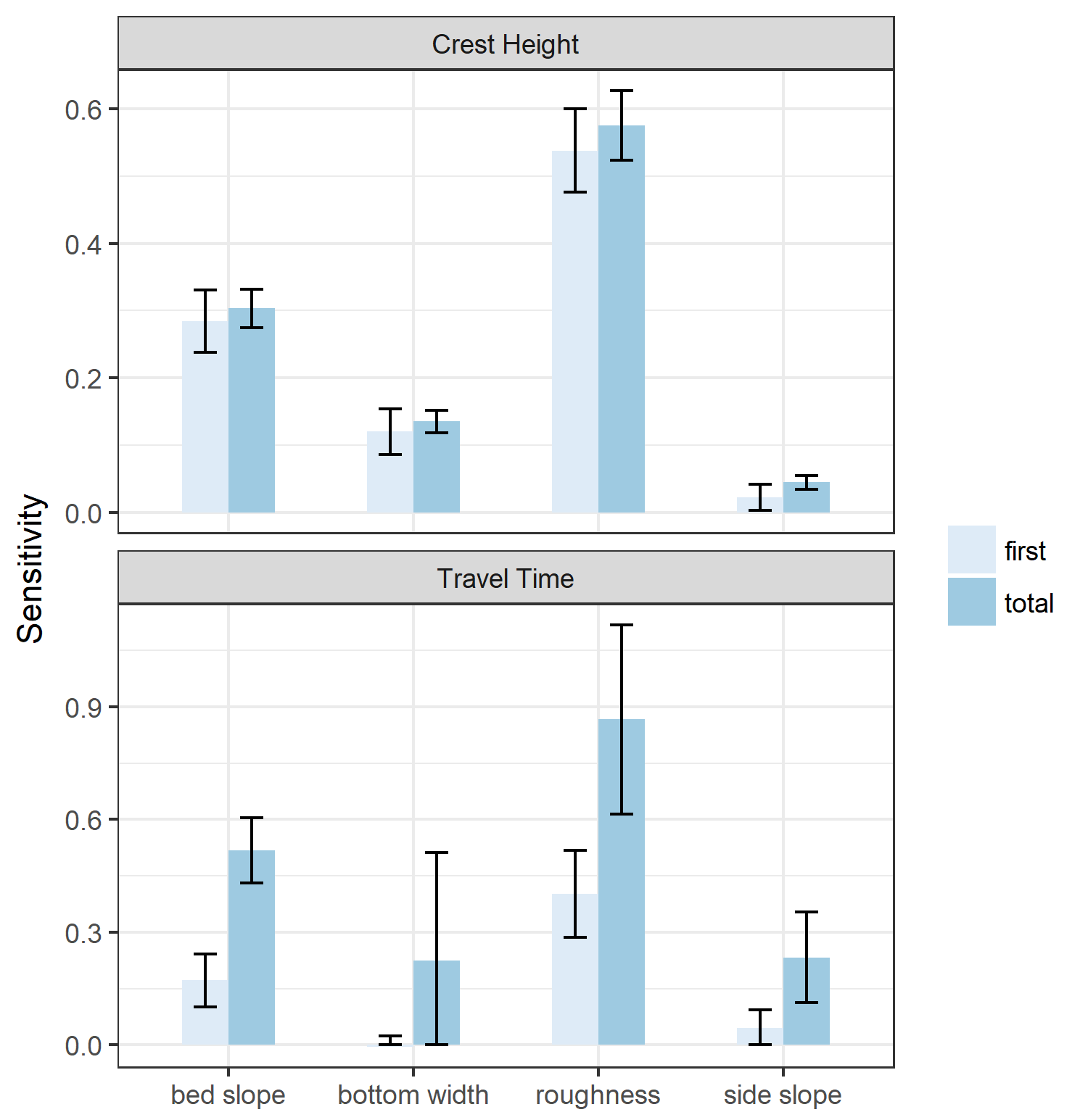
Note that the sensitivity indices cannot be negative, so a confidence interval that results in a negative value for the lower bound of a sensitivity index can be interpreted as equal to zero. The results are mostly as expected: bed slope and roughness have the most significant effect both on crest height and travel time. Side slope appears to have a low first-order effect on crest height, but becomes more significant when higher-order effects are taken into account (we’ll get to that in a minute). Bottom width has a significant effect on crest height, which is to be expected because a wider channel will by definition result in lower depths for the same flow. More surprising is that bottom width does not have a significant first-order effect on travel time, and potentially no significant higher-order effects. This is surprising, considering that the velocity of the flood wave is directly proportional to the area of flow under one-dimensional assumptions. Furthermore, there are significant higher-order effects from side slope, which similarly impacts flow velocities (since a larger side-slope results in larger flow areas). The uncertainty in the effect of bottom width is probably due to the fact that we explored a very large parameter range (50–200 feet). It might turn out that more iterations would clarify the effect of bottom width.
The “total” effects returned by sobol.analyze combine both the first-order
effect of the parameter and all higher-order effects. We can also explore
second-order effects of the parameters directly. Visualizing this is a little
harder, but I took a shot at it by mapping point sizes to the indices and
confidence intervals.
library(tidyr)
second.ind = list(
  "Crest Height" = setNames(
    as_data_frame(sensitivity.height$S2),
	unlist(problem$names)
  ) %>%
    mutate(var1 = unlist(problem$names)) %>%
    gather(var2, value, -var1),
  "Travel Time" = setNames(
    as_data_frame(sensitivity.time$S2),
	unlist(problem$names)
  ) %>%
    mutate(var2 = unlist(problem$names)) %>%
    gather(var1, value, -var2)
) %>%
  bind_rows(.id = "Output") %>%
  mutate(
    var1 = factor(var1, levels = unlist(problem$names),
	  labels = gsub(".", " ", unlist(problem$names), fixed = TRUE)),
    var2 = factor(var2, levels = unlist(problem$names),
	  labels = gsub(".", " ", unlist(problem$names), fixed = TRUE))
  )
second.conf = list(
  "Crest Height" = setNames(
    as_data_frame(sensitivity.height$S2_conf),
	unlist(problem$names)
  ) %>%
    mutate(var1 = unlist(problem$names)) %>%
    gather(var2, confint, -var1),
  "Travel Time" = setNames(
    as_data_frame(sensitivity.time$S2_conf),
	unlist(problem$names)
  ) %>%
    mutate(var2 = unlist(problem$names)) %>%
    gather(var1, confint, -var2)
) %>%
  bind_rows(.id = "Output") %>%
  mutate(
    var1 = factor(var1, levels = unlist(problem$names),
	  labels = gsub(".", " ", unlist(problem$names), fixed = TRUE)),
    var2 = factor(var2, levels = unlist(problem$names),
	  labels = gsub(".", " ", unlist(problem$names), fixed = TRUE))
  )

second.ind %>% left_join(second.conf) %>%
  mutate(
    lower = if_else(confint > value, 0, value - confint),
	upper = value + confint
  ) %>%
  ggplot() + aes(x = var1, y = var2) +
  geom_point(aes(size = upper, fill = Output), shape = 22) +
  geom_point(aes(size = value), shape = 22) +
  geom_point(aes(size = lower), shape = 22) +
  theme_bw() + xlab(NULL) + ylab(NULL) +
  scale_size_area("Effect", max_size = 20) +
  scale_fill_brewer(NULL, palette = "Accent") +
  coord_fixed()
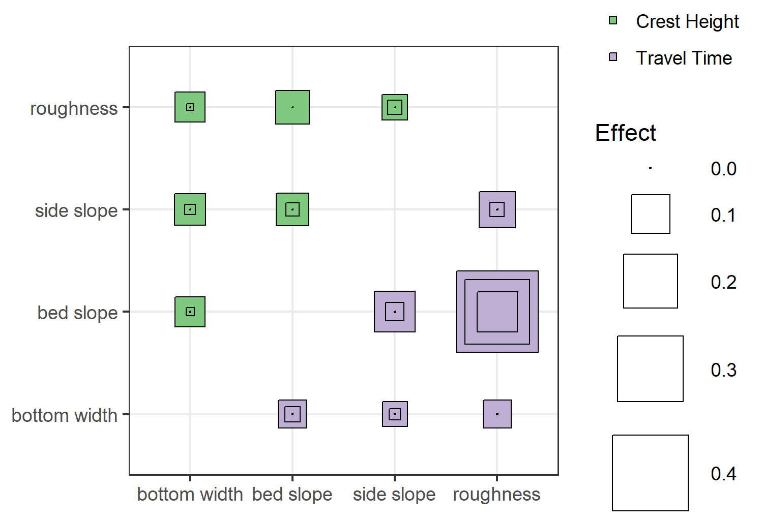
The above plot shows the second-order effects, with the inner/outer squares indicating the confidence intervals. Truthfully, I’m not that excited about this visualization, but it does illustrate relative effect sizes and uncertainty. Except for bed slope:roughness effect on travel time, the second-order effects of all interactions are potentially negligible (since the confidence interval includes zero). Also, while this doesn’t show up in the plot (because of the way I defined the size scale), some of my second-order indices are negative. This usually indicates a problem with sample size, i.e. the parameter space wasn’t sufficiently explored to get a good estimate of the effect.
Okay, that’s all I have for SALib and reticulate today. Now to rewrite
arcpyrextra to use
reticulate…
Comments
Want to leave a comment? Visit this post's issue page on GitHub (you'll need a GitHub account).